How fragile is acceleration?

Many optimizers in machine learning is descended from one line of mathematics:

Gradient descent is honest and slow. On a smooth, strongly convex function with condition number $\kappa$, it contracts the error by a factor of roughly $1 - 1/\kappa$ per step. Momentum methods — Polyak's heavy ball, Nesterov's accelerated gradient — improve this to $1 - 1/\sqrt{\kappa}$, a quadratic speedup in the condition number. When $\kappa$ is in the thousands, as it easily is, that is the difference between a coffee break and a lunch break.

The catch is stated in the fine print of every acceleration theorem: the gradient is assumed exact. In practice it never is. In machine learning contexts, gradients are often subsampled from data, quantized for communication, delayed in distributed systems, or — in adversarial settings — deliberately corrupted. And momentum, which works by extrapolating the past, extrapolates the errors of the past too.

Algorithms are dynamical systems

The productive move is to take the word "iteration" literally. A generalized momentum method — a family containing gradient descent, heavy ball, and Nesterov's method as parameter choices — can be written as a linear feedback system driven by gradient error:

where $\xi_k$ stacks the current and previous iterates and $w_k$ is whatever corruption the world supplies. Once the algorithm is a dynamical system, its sensitivity to noise stops being a vague worry and becomes a computable quantity — and which quantity depends on what you assume about $w_k$.

If the noise is random and unbiased, the iterates do not converge to the optimum; they settle into a stationary distribution around it, a cloud whose size is measured by the system's $H_2$ norm. On quadratics this is exact linear algebra: the variance solves the discrete Lyapunov equation

and $J$ — the noise amplification — can be read off for any stepsize and momentum you care to choose.

If instead the noise is adversarial — deterministic, finite energy, chosen by an opponent who knows your algorithm — the right measure is the $H_\infty$ norm: the worst-case amplification over all such disturbances. On quadratics this too admits a closed form, and the analysis produces something delightfully concrete: the worst-case disturbance itself, which turns out to be a decaying cosine tuned to the algorithm's own resonant frequency. An accelerated method rings like a bell, and the worst thing you can do to it is push at exactly that pitch.

The trade-off is a theorem

Here is the part I find genuinely beautiful. You might hope that some clever tuning gives both full acceleration and full robustness. It cannot. For the momentum family there is a Heisenberg-like inequality: the product of convergence speed and robustness is bounded below. Making $\rho$ (the rate) smaller forces $J$ (the amplification) larger. The frontier can be traced exactly, and designed on — choosing parameters that sit on the Pareto curve rather than at its fragile endpoint — but it cannot be escaped.

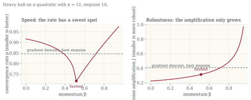
Average behavior is not the whole story either. Two algorithms with the same stationary variance can have very different tails, and in risk-sensitive applications the tails are what hurt. Entropic risk measures extend the analysis from means to rare events, which leads to risk-averse parameter selection: accept a slightly worse rate in exchange for provably thinner tails.

Speed times robustness is bounded below. The question is never "fast or robust?" — it is where on the frontier you choose to live.

Try it yourself

Everything above is easier to feel than to read. The momentum playground on this site runs these methods live: drag the momentum slider and watch $\rho$ improve while $J$ climbs; switch the gradient error to adversarial and watch a small, well-aimed cosine do what large random noise cannot. The quantities displayed are the exact $\rho$ and $J$ from the formulas above — computed, not eyeballed.

The full story, with the theorems this note compresses, is in the companion papers linked above: the Pareto frontier and robust tuning, the entropic-risk analysis, and the $H_\infty$ theory with its worst-case constructions.