Why heavy-tailed SGD leaves narrow basins

Companion to

The manuscripts

First exit time analysis of stochastic gradient descent under heavy-tailed gradient noise (NeurIPS, 2019)

A tail-index analysis of stochastic gradient noise in deep neural networks (ICML, 2019)

The heavy-tail phenomenon in SGD (ICML, 2021)

Stochastic gradient descent does not see the loss landscape; it sees the loss landscape plus noise. The standard mental model treats that noise as Gaussian — a diffusion — and a great deal follows from the model: SGD settles into a Gibbs-like distribution, it escapes a basin at a rate that is exponentially small in the barrier height, and so, left alone, it ends up in the deepest basin it can find.

The model is wrong in an interesting way. Measured on real networks, the gradient noise of SGD has heavy tails: its tail index $\alpha$ — the exponent in $\mathbb{P}(|\text{noise}| > t) \sim t^{-\alpha}$ — sits well below the Gaussian value of 2, often between 1 and 1.5, and it moves with the architecture, the stepsize and the batch size. A better continuous-time model is not a diffusion but a stochastic differential equation driven by an $\alpha$ -stable Lévy process,

dX_t = -\nabla f(X_t)\,dt + \varepsilon\, dL^{\alpha}_t ,

whose increments have infinite variance and whose sample paths jump. Everything that follows from the Gaussian model has to be rederived, and the first thing to change is where SGD ends up.

Climbing versus jumping

Take a basin of the loss with a minimum at the bottom, a barrier of height $\Delta$ on its rim, and a width $w$ — the distance from the minimum to the rim. For a Gaussian walker (noise scale $\varepsilon$ ), Kramers' law gives the mean time to escape:

\mathbb{E}[\tau] \asymp \exp\!\left(\frac{\Delta}{\varepsilon^2}\right).

The barrier height is in the exponent, the width is nowhere. A deep basin holds a Gaussian walker essentially forever, whatever its width, and a shallow one lets it go quickly, whatever its width.

For an $\alpha$ -stable walker the escape happens differently. It does not accumulate small steps until it has climbed the barrier; it waits for a single jump large enough to clear the rim in one go. The probability of such a jump at any given step is the tail probability of the noise beyond the distance $w$ , which is polynomial, and so is the waiting time:

\mathbb{E}[\tau] \asymp \left(\frac{w}{\varepsilon}\right)^{\alpha}.

Now the width is what matters and the height has disappeared — to leading order, the barrier can be as tall as you like. This is the Imkeller–Pavlyukevich asymptotics for Lévy-driven SDEs, and it is exactly what SGD inherits once its noise is heavy-tailed: the first-exit time of SGD, and of the SDE that models it, depends polynomially on the width of the basin rather than exponentially on its depth. Among several basins, the heavy-tailed walker leaves the narrow ones quickly and lingers in the wide ones; it does not care which is deepest. Since wide minima are the ones that tend to generalize, this is a mechanism — not a metaphor — connecting the tails of the gradient noise to the solutions SGD finds.

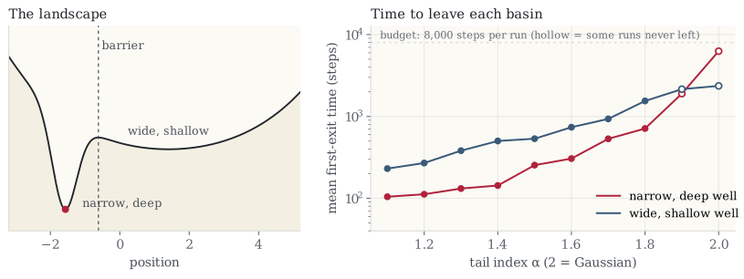
Left: a landscape with a narrow, deep well and a wide, shallow one. Right: the mean first-exit time from each well against the tail index, on a logarithmic scale; the narrow well is left in about a hundred steps for heavy tails and essentially never for Gaussian noise, while the wide well's exit time barely changes. — SGD on a landscape with a narrow, deep basin and a wide, shallow one, under α-stable gradient noise. For heavy tails (α near 1) the narrow basin is left within about a hundred steps and the wide one holds the iterate longer; as α approaches 2 the narrow basin becomes a trap. Sixty runs per point; hollow markers mean some runs never left within the budget.

The figure shows the two laws side by side on a toy landscape. At $\alpha = 1.1$ the narrow basin is left after about a hundred steps and the wide one takes twice as long; at $\alpha = 2$ the narrow basin holds the walker beyond the budget of the experiment while the wide one does not. Raising the barrier of the narrow basin changes the Gaussian prediction by orders of magnitude and the heavy-tailed exit time hardly at all.

Where the tails come from

It would be a weaker story if heavy tails were only a property of some datasets. They are not. Even with Gaussian data and a quadratic loss, the iteration of SGD is a random linear recursion of Kesten type,

x_{k+1} = M_k\, x_k + q_k ,

with a random multiplicative matrix $M_k$ that depends on the sampled batch. Such recursions have stationary distributions with power-law tails, and the tail index is not a property of the data: it is set by the ratio of the stepsize to the batch size, and by the stepsize schedule. SGD manufactures its own heavy tails, and the hyperparameters decide how heavy. Put the two results together and a dial appears: stepsize and batch size set $\alpha$ , and $\alpha$ sets which basins SGD can stay in.

A Gaussian walker climbs; a heavy-tailed one jumps. Exit times are exponential in the barrier height for the first and polynomial in the basin width for the second — and the stepsize-to-batch-size ratio decides which walker you have.

Try it yourself

The heavy-tails playground runs this experiment live: drag the tail index from 2 down to 1.1 and watch the run leave the narrow basin and settle in the wide one; raise the barrier and watch the Gaussian prediction explode while the measured heavy-tailed exit time stays put; narrow the well and watch the opposite. The readout sets the Monte Carlo exit times beside Kramers' formula and the single-jump law above.

The theorems are in the companion papers: the first-exit-time analysis of SGD under heavy-tailed noise, including the discretization error between SGD and its SDE; the measurements of the tail index of gradient noise in deep networks; and the heavy-tail phenomenon in SGD itself, with the stepsize-to-batch-size ratio controlling $\alpha$ .

Comments and corrections are welcome by email. More notes on the notes index, or subscribe via RSS.