Three ways to reach a saddle point

A surprising amount of modern machine learning is not a minimization. Distributionally robust learning minimizes over the model while an adversary maximizes over the data distribution; adversarial training does the same over perturbations; constrained problems become saddle-point problems the moment a Lagrange multiplier appears. The template is

and the first thing to know about it is that the obvious algorithm does not work.

Why descent-ascent spirals

Take the simplest strongly-convex–strongly-concave instance, $\mathcal{L}(x,y) = \frac{\mu}{2}x^2 + b\,xy - \frac{\mu}{2}y^2$, whose saddle point is the origin. Gradient descent-ascent — a descent step in $x$ and an ascent step in $y$, simultaneously — is the linear iteration $z_{k+1} = (I - \eta F)\,z_k$ with

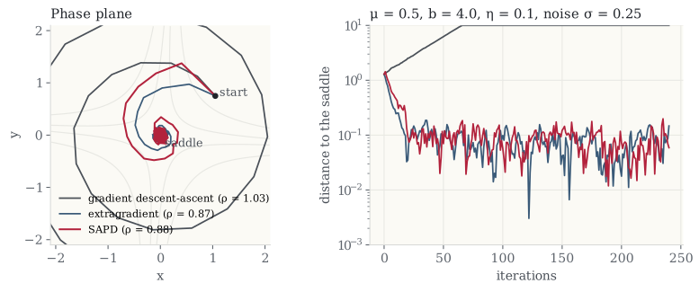
whose eigenvalues are $1 - \eta\mu \pm i\,\eta b$. The coupling $b$ shows up as a pure rotation. A gradient step taken on a rotation always lands a little farther from the center, and the modulus $\sqrt{(1-\eta\mu)^2 + \eta^2 b^2}$ exceeds one as soon as $\eta > 2\mu/(\mu^2 + b^2)$. When the coupling dominates the curvature — the typical case — descent-ascent either spirals outward or converges only with a stepsize so small that it barely moves.

The two cures both amount to damping the rotation. Extragradient looks one step ahead: it takes a trial step, evaluates the gradient there, and uses that gradient for the real step. The look-ahead cancels the rotation to first order at the price of a second gradient per iteration. The accelerated primal–dual approach does the same with momentum: SAPD extrapolates the dual gradient,

with one gradient of each kind per iteration, and the momentum parameter $\theta$ plays the role the look-ahead plays for extragradient.

Stochastic gradients, and the price of speed

In learning problems the gradients are stochastic, and then convergence is not the whole story. Because each method is a linear system driven by the gradient noise, two numbers describe it exactly. The convergence rate $\rho$ is the spectral radius of its iteration matrix. The robustness is a number $J$: the stationary root-mean-square distance to the saddle when every gradient carries unit-variance noise — the $H_2$ norm of the system, which comes out of the discrete Lyapunov equation $X = AXA^{\top} + BB^{\top}$. With noise of scale $\sigma$, the run cannot converge; it hovers at a floor of about $\sigma J$. Both $\rho$ and $J$ can be computed for any choice of stepsizes and momentum.

Computing them reveals the same tension that governs momentum methods for minimization: turn the stepsize up and every $\rho$ falls while every $J$ rises. SAPD makes the trade-off designable. Its analysis gives, for a target rate, the stepsizes and momentum that achieve it, and shows that the rate and the noise amplification cannot be minimized together — there is a Pareto frontier between them, which can be traced and chosen on. In expectation that is the whole story; for a single run it is not, because an algorithm that is fine on average can still have fat tails. High-probability and risk-averse guarantees for SAPD address exactly that, certifying the run you actually get rather than the average run. And the same machinery extends beyond the convex–concave case: SAPD+ uses the method as an inner solver to reach the best known complexity for non-convex–concave problems.

Reaching a saddle point is a question of damping a rotation; doing it fast and doing it quietly pull in opposite directions, and the frontier between them can be computed.

Try it yourself

The saddle-point playground races the three methods from the same start with sliders for the coupling, the curvature, the stepsize, the momentum and the noise. The table underneath gives each method's exact $\rho$ and $J$ beside the measured distance of the noisy run; press Coupling dominates to watch descent-ascent spiral out, then drag the stepsize to watch the frontier.

The theory is in the companion papers: SAPD and its rate–robustness analysis, the high-probability and risk-averse guarantees for a single run, and SAPD+ for non-convex–concave problems.