Why random reshuffling beats SGD

Stochastic gradient descent, as analyzed, picks a component function at random at every step. Stochastic gradient descent, as implemented, does nothing of the kind: it shuffles the training set once, sweeps through it in that order, and shuffles again. The sampling is without replacement, in epochs. The practice is universal, the folklore says it is faster, and until recently the theory had nothing to say about it, because the samples within an epoch are not independent and the usual martingale arguments fall apart.

The theory now says the folklore is right, and says by how much.

Two rates

Consider a finite sum $f(x) = \frac{1}{n}\sum_{i=1}^{n} f_i(x)$ with $f$ strongly convex and the $f_i$ smooth, and a diminishing stepsize $\alpha_k = \Theta(1/k^s)$ held fixed during epoch $k$. For SGD with replacement — independent indices at every step — the best possible rate is

a lower bound for stochastic approximation that no stepsize schedule can beat. For random reshuffling — a fresh uniformly random permutation at every epoch — the rate is

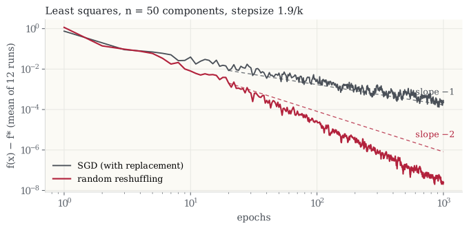
which approaches $1/k^2$ as $s \to 1$. Not a better constant: a better exponent. On a log–log plot of error against epochs, SGD is a line of slope $-1$ that it cannot leave, and reshuffling is a line of slope $-2$.

Where the factor comes from

The mechanism is visible in a single epoch. Write the full gradient at the start of epoch $k$ as $\nabla f(x)$. With replacement, the $n$ sampled gradients add up to $n\,\nabla f(x)$ only on average; the sum has a fluctuation of order $\sqrt{n}$ times the gradient noise, and the epoch's total step is off by a term of order $\alpha_k$. That error is paid at every epoch, it never cancels, and summing it is what pins SGD to $1/k$.

Under reshuffling, every component appears exactly once in the epoch, so the first-order sum is $\sum_i \nabla f_i(x) = n\,\nabla f(x)$ exactly. The sampling noise cancels within the epoch. What remains is the fact that the gradients were evaluated at points that drift during the epoch rather than at $x$ itself, and that error is of order $\alpha_k^2$ — one order smaller. Measured directly, the error of one epoch's step decays like $\alpha_k$ with replacement and like $\alpha_k^2$ under reshuffling; squaring the per-epoch error is what squares the rate.

The second-order error is where the analysis earns its keep. It is not independent across epochs, and its expectation over the permutation is not zero. The proof decouples it into a term that is independent across epochs and a term dominated by $\alpha_k^2$, and then controls the whole sequence with a law of large numbers, which gives the rate with probability one rather than only in expectation. A fixed cyclic order already removes the within-epoch sampling noise — that alone takes the incremental gradient method out of the $1/k$ regime — but the randomness of the permutation is what makes the remaining error average out from epoch to epoch, and on well-conditioned problems the reshuffling curve is steeper still than the theorem's $1/k^2$.

Sampling with replacement pays for its noise at every step; reshuffling pays once per epoch, at second order — and that squares the rate.

The same question — does the order of visiting matter, and does randomizing it help — has a parallel answer for coordinate descent, where a fixed cyclic order can provably beat random sampling on some problems and random permutations beat both on others.

Try it yourself

The reshuffling playground runs the experiment above with sliders for the number of components, the stepsize exponent $s$ and the amount of noise at the optimum. The reference slopes move with $s$ — $-s$ against $-2s$ — so the squaring is visible as a change of slope rather than a change of constant, and a second chart measures the error of one epoch's step directly, which is where the cancellation lives.

The theorems, with their constants and the probability-one statements, are in the companion papers: the reshuffling analysis itself, the convergence rates of the incremental gradient and incremental Newton methods under a fixed order, and the coordinate-descent counterpart.