Can momentum survive a delay?

Accelerated methods are the workhorses of large-scale optimization, and their theory rests on a small assumption that distributed systems break all the time: that the gradient used at step $k$ is the gradient at the current point. When several workers compute gradients in parallel and a shared iterate moves on while they work, the gradient that arrives at step $k$ describes the iterate as it was some steps earlier. It is stale. The question of this note, and of the paper it accompanies, is whether momentum methods can stay accelerated on stale gradients, and if so, how.

The answer has two halves. Heavy ball and Nesterov's method cannot, however their parameters are retuned. A third method can, by matching one of its parameters to the delay. The playground lets you run all three.

The setting: a fixed delay, no idling

Fix an integer delay $\tau \ge 1$ . We minimize an $L$ -smooth, $\mu$ -strongly convex function $f$ with condition number $\kappa = L/\mu$ , and at iteration $k$ the oracle returns $\nabla f(y_{k-\tau})$ : the gradient at the point queried $\tau$ iterations ago. The method is non-idling: it takes a step with every gradient that arrives, rather than waiting until a gradient at its current point is available.

This is an idealization of asynchronous optimization, chosen to isolate one effect. Real delays vary across workers and iterations, and real gradients are noisy; here the delay is constant and the gradient is exact, so that whatever changes is due to staleness alone.

One can always match the delay by waiting. Run Nesterov's method, make one update every $\tau + 1$ iterations when a fresh gradient has arrived, and idle in between. This reaches accuracy $\varepsilon$ in $O\big((\tau+1)\sqrt{\kappa}\log(1/\varepsilon)\big)$ iterations, and a lower bound of Arjevani, Shamir and Srebro says that no first-order method using $\tau$ -delayed gradients, in high enough dimension, can do better than

\Omega\!\big((\tau+1)\sqrt{\kappa}\,\log(1/\varepsilon)\big)

iterations, even on quadratics. So the factor $\tau + 1$ is the price of the delay, and it cannot be avoided. The waiting method pays it by discarding $\tau$ of every $\tau+1$ gradients. The question is whether a method that uses every stale gradient can reach the same scaling: an iteration complexity proportional to $\tau\sqrt{\kappa}$ , rather than to $\tau\kappa$ , which is what delayed gradient descent achieves.

One family, three dials

All the methods in this note are members of the generalized momentum method with a delay:

y_k = x_k + \nu\,(x_k - x_{k-1}), \qquad x_{k+1} = x_k - \alpha\,\nabla f(y_{k-\tau}) + \beta\,(x_k - x_{k-1}).

Here $\alpha > 0$ is the stepsize, $\beta \ge 0$ the momentum, and $\nu \ge 0$ the extrapolation: how far ahead of the current iterate the gradient is queried. Heavy ball is $\nu = 0$ (query at the iterate itself), and Nesterov's method is $\nu = \beta$ (query at the momentum-extrapolated point). Every parameter is constant; the delay is the only thing that changes from the classical recursion. The methods start from a constant history $x_{-\tau-1} = \dots = x_0$ .

What "accelerated" means here

On a quadratic $f(x) = \tfrac12 x^\top Q x$ the recursion decouples along the eigenvectors of $Q$ , and along an eigenvector with eigenvalue $\lambda$ the error satisfies a linear recurrence of order $\tau + 2$ . Its characteristic polynomial is

P_{\tau,\delta}(z) = z^{\tau}(z-1)(z-\beta) + \delta\,\big((1+\nu)\,z - \nu\big), \qquad \delta = \alpha\lambda .

The method converges on every quadratic with spectrum in $[\mu, L]$ if and only if

\rho(\alpha,\beta,\nu) = \sup_{\lambda \in [\mu, L]} \max\{|z| : P_{\tau,\alpha\lambda}(z) = 0\} < 1,

and then $\|x_k - x^\star\| \le c_k\,\rho^k$ with $c_k$ growing at most polynomially. So $\rho$ is the rate, and $1 - \rho$ , the spectral gap, is the quantity to maximize over the parameters. Without delay, gradient descent has $1 - \rho \asymp 1/\kappa$ , while heavy ball and Nesterov's method have $1 - \rho \asymp 1/\sqrt{\kappa}$ . That square root is what accelerated means: on a plot of $\log(1-\rho)$ against $\log\kappa$ , an accelerated method is a line of slope $-\tfrac12$ , and a non-accelerated one a line of slope $-1$ .

For each delay, let $\rho^\star_{\mathrm{HB}}(\tau,\kappa)$ and $\rho^\star_{\mathrm{NAG}}(\tau,\kappa)$ be the smallest rates heavy ball and Nesterov's method can reach over all stable choices of their two parameters. This is the fairest possible comparison: each classical method is allowed to know the delay and to retune itself for it.

Delay kills classical momentum

The paper's first main result is that retuning does not help:

1 - \rho^\star_{\mathrm{HB}}(\tau,\kappa) = O_\tau(\kappa^{-1}) \;\;(\tau \ge 1), \qquad 1 - \rho^\star_{\mathrm{NAG}}(\tau,\kappa) = \begin{cases} \Theta(\kappa^{-2/3}) & \tau = 1,\\[2pt] O_\tau(\kappa^{-1}) & \tau \ge 2, \end{cases}

as $\kappa \to \infty$ , with constants that may depend on $\tau$ but not on $\kappa$ . Heavy ball loses the square root at the first step of delay. Nesterov's method is more robust: with a one-step delay its best gap scales like $\kappa^{-2/3}$ , which is strictly between the accelerated and the non-accelerated exponents, and the paper shows this exponent is sharp. From two steps of delay on, it too is non-accelerated. Both statements are about the full range of stable constant parameters: there is no clever stepsize or momentum to find.

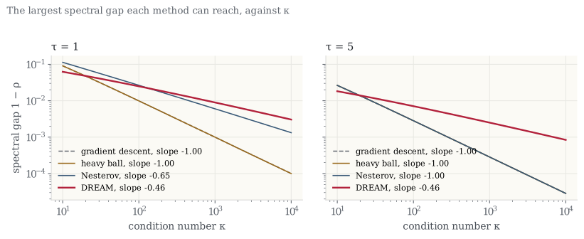
The numbers agree. Tuning each method numerically at each $\kappa$ and fitting the slope of $\log(1-\rho^\star)$ against $\log\kappa$ gives, from the paper's experiments,

Method	τ = 1	τ = 5	τ = 10	τ = 100
Gradient descent	−1.00	−1.00	−1.00	−1.00
Heavy ball	−1.00	−1.00	−1.00	−1.00
Nesterov	−0.66	−1.00	−1.00	−1.00
DREAM	−0.48	−0.49	−0.49	−0.49

The last row is the method introduced next.

Two log-log panels of the spectral gap against the condition number, for delays one and five. Gradient descent, heavy ball and Nesterov, each numerically tuned, follow lines of slope near minus one, except Nesterov at delay one with slope near minus two thirds; DREAM follows a line of slope near minus one half in both panels. — The largest spectral gap each method can reach, against κ, for delays τ = 1 and τ = 5 (numerically tuned gradient descent, heavy ball and Nesterov; DREAM with its formula). The slopes are fitted over κ ≥ 100.

Why: the query must lead the iterate by more than the delay

Here is a way to read what goes wrong, and what fixes it. Near convergence, along the slow direction of an accelerated method, the iterates move with a nearly constant velocity $v$ per step, so $x_k \approx x_{k-\tau} + \tau v$ . The gradient available at step $k$ was taken at

y_{k-\tau} = x_{k-\tau} + \nu\,(x_{k-\tau} - x_{k-\tau-1}) \approx x_k + (\nu - \tau)\,v .

With $\nu = \tau$ the stale query point coincides, to first order, with the current iterate; with $\nu > \tau$ it lies slightly ahead of it, which is exactly where Nesterov's method queries without delay. With $\nu \le \tau$ the method is steering by a gradient taken behind where it stands. Heavy ball has $\nu = 0$ and Nesterov's method has $\nu = \beta < 1$ , so neither can get ahead of a delay of one step or more.

The paper makes this precise. For the parameterization $\alpha = \delta_L/L$ , $\beta = 1 - 2\sqrt{\delta_L}/\sqrt{\kappa}$ , the rate satisfies $\rho \le 1 - \gamma/\sqrt{\kappa}$ for every $\gamma < \sqrt{\delta_L}$ and all large $\kappa$ , provided the limiting polynomial

P_\infty(z;\delta,\nu) = z^{\tau}(z-1)^2 + \delta\,\big((1+\nu)z - \nu\big)

has all its roots inside the unit circle for every $0 < \delta \le \delta_L$ ; and this is impossible unless $\nu > \tau$ . The extrapolation has to exceed the delay. Since $\nu$ is tied to $\beta$ in Nesterov's method and to zero in heavy ball, the only way out is to let $\nu$ be a third, independent dial.

DREAM

The paper's method, delay-resistant acceleration with momentum, is the generalized momentum method with

M = 2\tau + 1, \qquad \alpha = \frac{1}{M^2 L}, \qquad \beta = 1 - \frac{2}{M\sqrt{\kappa}}, \qquad \nu = M - \tfrac12 = 2\tau + \tfrac12 .

The extrapolation is a little more than twice the delay. The stepsize and the momentum are exactly Nesterov's for a problem whose smoothness constant has been inflated from $L$ to $M^2 L$ , so that its condition number reads $M^2\kappa$ ; the extrapolation is the new ingredient. On quadratics the rate is

\rho \;\le\; 1 - \frac{1}{2M\sqrt{\kappa}} = 1 - \frac{1}{2(2\tau+1)\sqrt{\kappa}}

for all sufficiently large $\kappa$ . The square root is back, and the delay enters only through the constant $2\tau+1$ , as the lower bound says it must. For $\tau = 1$ there is a sharper, fully explicit tuning whose worst-case rate is exactly $1 - 1/(2\sqrt{\kappa})$ for every $\kappa \ge 1$ , and the paper shows that the coefficient $\tfrac12$ cannot be improved by any constant-parameter method of this family.

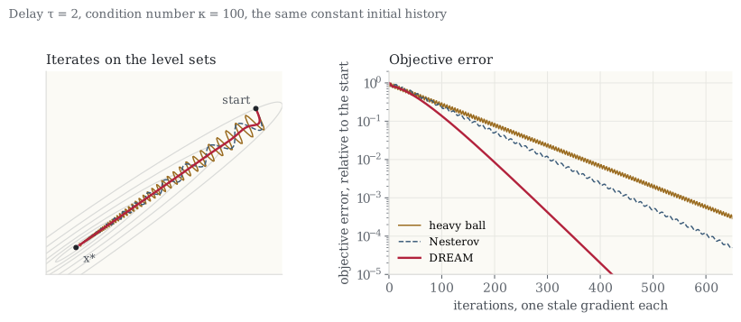
Left: the iterates of heavy ball, Nesterov and DREAM on the elliptical level sets of a quadratic with condition number 100 under a delay of two, from a common start; the two classical methods zigzag down the valley while DREAM goes nearly straight. Right: the normalized objective error against iterations on a log scale, with DREAM's line far steeper. — The race at τ = 2 and κ = 100, the playground's opening configuration. Heavy ball and Nesterov use the parameters that minimize their worst-case rate for this delay; DREAM uses its formula. Every method takes one step per stale gradient.

Is the constant $1/(2M)$ the best possible? Not quite. The paper solves the design problem exactly: among all $\nu > \tau$ , the largest rate coefficient this analysis can certify is $c^{\mathrm{crit}}_\tau$ , attained at an extrapolation $\nu^{\mathrm{crit}}_\tau \approx 1.72\,\tau$ for large delays, and $c^{\mathrm{crit}}_\tau \approx 0.74/\tau$ . The simple choice above keeps more than a third of that. It was kept because its parameters also work beyond quadratics, which is the second half of the paper.

Beyond quadratics

Stability of the characteristic polynomial says nothing, by itself, about a non-quadratic $f$ : the gradient is then a nonlinear map, and a method can be stable on every quadratic in a class and still fail on some strongly convex function in it, as heavy ball famously does. To carry the rate over to all $L$ -smooth, $\mu$ -strongly convex functions, the paper writes the delayed method as a feedback loop between a linear system with delay and the gradient map, and certifies the rate with an integral quadratic constraint of Zames–Falb type, weighted by the rate and taken over a finite horizon. These constraints capture relations between gradients at different points along the trajectory, which pointwise smoothness and convexity inequalities miss.

The outcome is a theorem with the same shape as the quadratic one. For every fixed delay and every $c \in (0, 2/3)$ , there is a threshold $\kappa_0(\tau, c)$ such that for $\kappa \ge \kappa_0$ , DREAM satisfies

\|x_k - x^\star\| \le C\,\Big(1 - \frac{c}{M\sqrt{\kappa}}\Big)^{k}

on every function in the class, from every starting history. With the constant-history start the threshold and the prefactor are polynomial in $M$ : $\kappa_0 = O(M^8)$ and $C = O(M^5\kappa^2)\,\|x_0 - x^\star\|$ . Reaching accuracy $\varepsilon$ therefore takes

O\!\Big(M\sqrt{\kappa}\,\big[\log(\mu R^2/\varepsilon) + \log M + \log\kappa\big]\Big)

iterations, which is the lower bound up to the logarithms. What makes the certificate usable is that it is analytic: as $\kappa \to \infty$ the frequency-domain condition reduces to the positivity of an explicit trigonometric polynomial, and the finite- $\kappa$ case is handled by estimates near and away from frequency zero. There is no semidefinite program to solve for each delay and no numerical search over frequencies; the parameters are written down, and the proof holds for every $\tau$ at once.

For smooth convex functions that are not strongly convex, DREAM serves as the inner solver of an accelerated proximal-point scheme in the style of Catalyst. When the target accuracy is small enough, the total number of stale-gradient updates is $\widetilde O\big((\tau+1)\sqrt{LR^2/\varepsilon}\big)$ , again the delayed lower bound up to logarithms.

What the experiments add

Two findings go beyond the theorems. On $\ell_2$ -regularized logistic regression, a smooth strongly convex problem that is not quadratic, the number of iterations needed to reach a fixed accuracy grows like $\sqrt{\kappa}$ for DREAM and drifts toward $\kappa$ for heavy ball and Nesterov's method as the delay grows, reproducing the quadratic picture. And the delay does not have to be known exactly: designing the parameters for a conservative upper bound $\hat\tau = 10$ while the true delay is anywhere from $0$ to $10$ keeps the $\sqrt{\kappa}$ scaling and changes only the constant in front. In practice, overestimating the delay is safe; underestimating it is what the first half of the note warns against.

Momentum alone cannot look far enough ahead to make up for a stale gradient. Extrapolate the gradient query by more than the delay and the acceleration survives, at a cost of a factor 2τ + 1 in the rate, which no method can avoid.

What the theory leaves open is also clear: delays that vary over time or across workers, stochastic gradients, and non-convex objectives. The lesson so far is that staleness need not cost the square root, provided the dynamics of the method are matched to the structure of the delay.